What are Reed-Solomon codes? What even is a “code” in this context??? That’s the question I kept asking myself.

I had no idea what “coding theory” was… yet I kept coming across those “RS codes”. So I decided to dig in.

Let’s start with a high level overview before going deeper. I’ll try to keep things simple and avoid copy-pasting the same definitions you see everywhere.

From now on, I’ll mostly use “RS” as shorthand for Reed-Solomon codes, because typing it out every time is tiring 😁

The big picture

What are RS codes?

Forget about the word “code” for a second, it can be confusing.

RS is essentially a way to correct errors when transmitting data. That’s it. Simple.

Practical Applications

RS codes are everywhere:

• QR codes: error correction in scanning
• CDs and DVDs: recovering scratched data
• Space communication: handling signal errors from deep space
• Your hard drive: data redundancy in storage systems

A common example: QR codes. When you scan a QR code, RS helps ensure the data is correctly interpreted. That’s why, even if the image has a small scratch, you can still retrieve the data through error correction.

How do they work?

By adding redundancy to the data.

The core idea is to expand the data being sent, making it more resilient to errors. If some parts of the transmission get corrupted, the extra information helps reconstruct the original message. So yes, the data will be bigger but at least it will be correctly transmitted.

Going back to our QR code example, the image consists of many black and white squares. Imagine you have a QR code ready to scan, and you count 400 squares in total.

The reality is that your camera doesn’t actually need all 400 squares to understand the data. It might only require 300 (for example). The extra squares are there to compensate for potential data loss—such as a damaged or partially obstructed image.

Finally, an RS decoding algorithm takes these squares and reconstructs the correct data, even if some are missing or incorrect.

Coding theory

Here’s the Wikipedia definition:

Coding theory is the study of the properties of codes and their respective fitness for specific applications. Codes are used for data compression, cryptography, error detection and correction, data transmission and data storage

Before getting technical, let’s define some key terms:

• code: a set of symbols used to represent information
  • Example: The English alphabet is a code, just like the Greek alphabet.
  • In mathematics, the digits from 0 to 9 can also be considered a code.
• codeword: a specific sequence of symbols from the code
  • Example: In the English alphabet, “computer” is a codeword, it consists of eight symbols from the alphabet.
  • Symbols can be repeated, so “teddav” is also a valid codeword.
  • In the case of digits, any number (e.g., 2734) is a codeword.

Does that make things clearer? 💡

By the way, when discussing RS codes, you’ll often see the term “alphabet.” In this context, it is simply another word for “code”, it refers to the set of symbols being used.

RS codewords

What about code and codeword in RS?

In Reed-Solomon codes, we use prime finite fields, meaning our data is represented as an array of numbers within the field.

The length of a codeword is pre-determined by both the sender and receiver so that both parties know what to expect. Later, we’ll see how RS codes encode both the message and redundancy.

Example:

If we decide to use the field $\mathbb{F}_{113}$:

• our code (or alphabet) will be all the numbers from 0 to 112 (included).
• The codeword length is chosen in advance. Suppose we decide on a length of 9, then a possible codeword could be: [106, 57, 14, 109, 66, 99, 46, 28, 8]

Let’s get real (or finite)

Ok that’s terrible. I’m sorry for the “joke”, but I’m going to leave it anyway 🥲

First, I’ll define the key parameters we’re going to use, and then we’ll dive into the technical details to see how everything actually works.

Parameters

• n → Length of the codeword. This is the entire transmitted data, including redundancy.
• k → Length of the message. This is the actual message the sender wants to transmit, without redundancy.

In simple terms: if we want to send a message of length k, we must expand it to length n.

That means n - k symbols are used for errors correction, and the maximum number of errors we can correct is $\frac{n-k}{2}$

Encode messages

For all this magic to work, we need polynomials.

The core idea of RS codes is:

1. Encode the original message as a polynomial.
2. Evaluate the polynomial at n points.

That’s it! 😂 I swear it’s really that simple.

I’ll provide examples soon, but first, let’s build some intuition about why RS codes work.

Why does it work?

RS codes rely on the principle that a polynomial of degree d is uniquely determined by d+1 points. If some points are corrupted, we can still reconstruct the original polynomial, as long as we have at least d+1 valid points.

In the case of RS codes, we need slightly more than d+1 points to ensure we are interpolating the correct data.

Example:

Say n = 10 and k = 5. We could interpolate two different polynomials:

• One from points 1 to 5
• Another from points 6 to 10

Without additional constraints, there’s no way to determine which one is correct.

A note on Sagemath

A quick tip for using SageMath: I find it easiest to run their official Docker image, sagemath/sagemath.
See this article for help: https://teddav.github.io/sagemath

Polynomial interpolation

If you’re not familiar with polynomial interpolation, there are plenty of great resources online, so I won’t go into full detail here.

The simplest example:

For a line (a degree-1 polynomial), two points are enough to determine its equation. If we have a third point and it doesn’t lie on the line, we know there’s an error.

The same principle applies to higher-degree polynomials. If we have enough correct points, we can uniquely reconstruct the original polynomial. The interpolation algorithm itself isn’t particularly complex, and if you’re a visual learner, I highly recommend DrWillWood’s video.

That said, here’s a small Sage script you can experiment with:

F = GF(101)
R = F['x']

# we want a degree 5 polynomial
d = 5

# we pick 6 random points (d + 1)
# these will be our `y` values
ys = [F.random_element() for _ in range(d + 1)]
print("y values: ", ys)

# our `x` values will be 0 to d
points = [(x,y) for (x,y) in enumerate(ys)]

P = R.lagrange_polynomial(points)
print("points1: ", points)
print("P1: ", P)

# now we add a few more points
# these are still on the same polynomial
points.append((6, P(6)))
points.append((7, P(7)))

# if we interpolate again, we get the same polynomial
P2 = R.lagrange_polynomial(points)
assert P2 == P
print("points2: ", points)
print("P2: ", P2)

# finally we modify just 1 points
points[0] = (0,0)
P3 = R.lagrange_polynomial(points)
print("points3: ", points)
print("P3: ", P3)

Here’s what gets printed:

y values:  [25, 58, 9, 8, 85, 75]

points1:  [(0, 25), (1, 58), (2, 9), (3, 8), (4, 85), (5, 75)]
P1:  96*x^5 + 29*x^4 + 40*x^3 + 14*x^2 + 56*x + 25

points2:  [(0, 25), (1, 58), (2, 9), (3, 8), (4, 85), (5, 75), (6, 28), (7, 13)]
P2:  96*x^5 + 29*x^4 + 40*x^3 + 14*x^2 + 56*x + 25

points3:  [(0, 0), (1, 58), (2, 9), (3, 8), (4, 85), (5, 75), (6, 28), (7, 13)]
P3:  48*x^7 + 70*x^6 + 99*x^5 + 81*x^4 + 35*x^3 + 19*x^2 + 9*x

You can see how the last polynomial is completely different even though we just changed 1 point.

Encoding

Now comes the fun part!

I’ll use Sage to encode data using Reed-Solomon codes. Once that’s done, we’ll move on to decoding, which is a bit trickier.

For this example, we’ll encode the message “TEDDAV”.

• Since k represents the length of our message, here we have k = 6, meaning the polynomial will have degree 5.
• The encoded codeword will have length n = 13. Why 13? No special reason, I just picked it randomly 😊

Before jumping into the code, let’s quickly recap the encoding process:

1. Convert each letter in our message into its corresponding numerical value.
2. Use these values as coefficients to construct a polynomial P.
3. Introduce redundancy by evaluating P at 13 different points (from 0 to 12). This gives us our final codeword.

F = GF(101)
R = F['x']

message = "TEDDAV"
message = [ord(c) for c in message]
print("message", message)

k = len(message)
n = 13

# we define our polynomial P from the message
P = R(message)
print("P: ", P)

# we evaluate P at n points to get our codeword
codeword = [P(i) for i in range(n)]
print("codeword: ", codeword)

message:  [84, 69, 68, 68, 65, 86]
P:  86*x^5 + 65*x^4 + 68*x^3 + 68*x^2 + 69*x + 84
codeword:  [84, 36, 83, 16, 10, 36, 81, 65, 61, 10, 42, 90, 9]

Now that our codeword is ready, it can be transmitted. Upon receiving it, the recipient will check for errors.

Decoding without error

The receiver already knows the parameters:

• k = 6 → the original message length
• n = 13 → the total length of the codeword

Since they expect a codeword of length 13 and want to recover a message of length 6, they follow this simple verification process:

1. Interpolate a polynomial P from the received points.
2. Check its degree:
   • If the degree is 5 → The codeword is valid, and we can recover the message.
   • If the degree is greater than 5 → An error occurred.

Let’s check:

# check if codeword is valid
codeword = [84, 36, 83, 16, 10, 36, 81, 65, 61, 10, 42, 90, 9]
points = [(x,y) for (x,y) in enumerate(codeword)]
P = R.lagrange_polynomial(points)

if P.degree() == 5:
    print("We can get the message!")
else:
    print("There was an error :(")
    exit()

coefficients = P.coefficients(sparse=False)
recovered_message = [chr(m) for m in coefficients]
print("message: ", recovered_message)

Output:

We can get the message!
message:  ['T', 'E', 'D', 'D', 'A', 'V']

Success! 🎉🥳🍾

We’ve successfully sent and decoded a Reed-Solomon encoded message.

Now, just for fun, let’s introduce an error and see how we can still recover the message.

Decoding

There are several ways to decode Reed-Solomon codes. Today we’ll use the Berlekamp–Welch algorithm.

To make things easier, I’ll start with this example from Wikipedia and break it down step by step.

Once we understand the process, we’ll apply the same algorithm to our own example to recover the original message.

Here’s the Wikipedia example:

Setup

We define the following parameters:

• Alphabet: $\mathbb{F}_{929}$ (all numbers from 0 to 928)
• Codeword length: n=7
• Message length: k=3
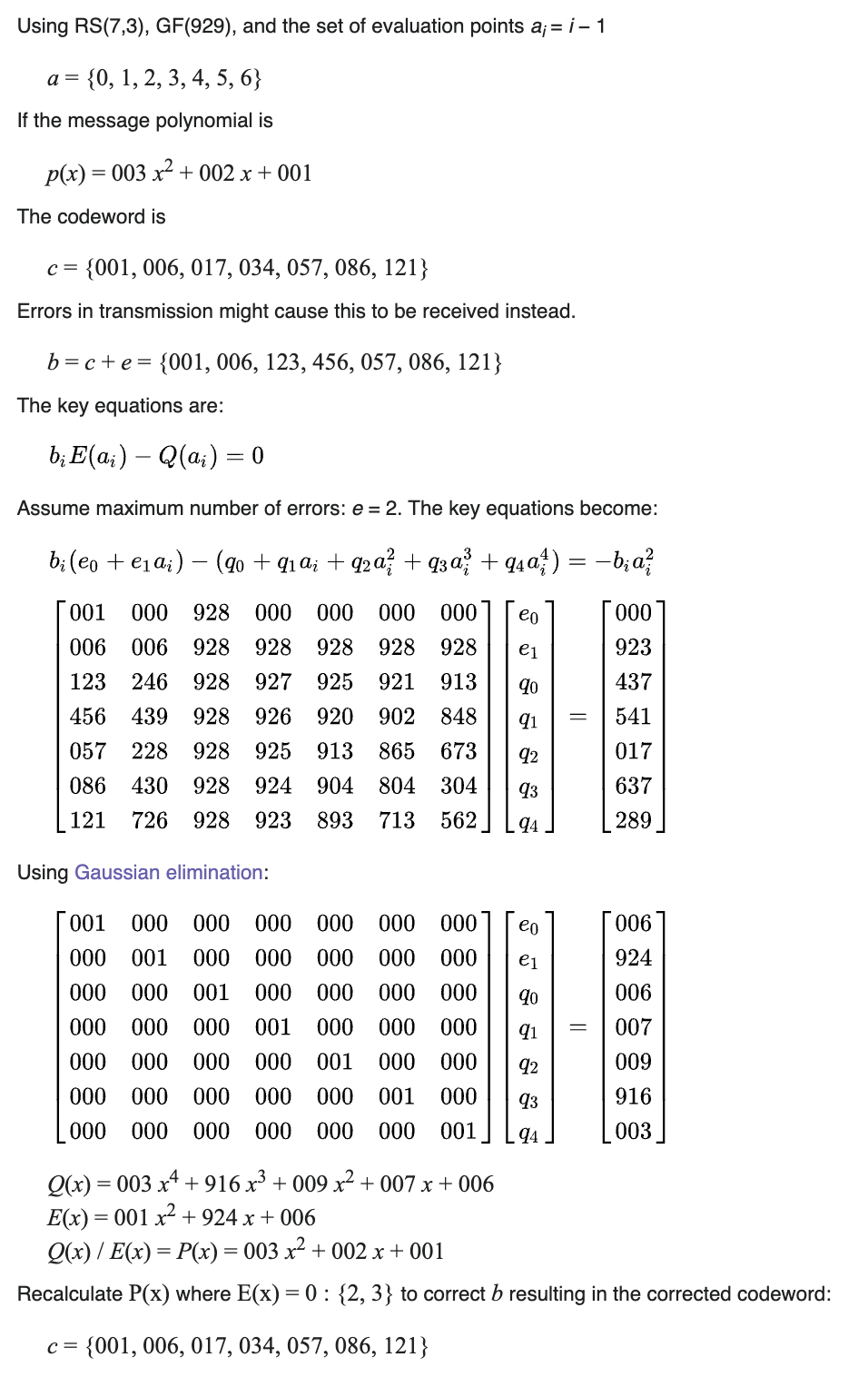
• Message: [1, 2, 3]
• Evaluation points (referred to as $a_i$): $a_i=0,1,2,3,4,5,6$

How many errors can we correct?

The formula is:

So we can correct up to 2 errors.

The message polynomial is:

We construct it simply by using the message values as coefficients.

The codeword is generated by evaluating $P(x)$ at $a_i$:

c = { P(0), P(1), … , P(6) } = { 1, 6, 17, 34, 57, 86, 121 }

The receiver receives b (a possibly corrupted version of c), and their task is to determine if there are errors and recover the original message.

Error polynomial

To detect and correct errors, we introduce an error polynomial $E(x)$, which satisfies the following conditions:

• $E(x)$ has degree equal to the maximum number of errors: degree = 2
• The leading coefficient is 1, so $E(x)=x^2+e_1x+e_0$
• $E(a_i)=0$, if there’s an error at index i(we don’t know these locations yet)

The key equation that must hold for all received values $b_i$ is:

We have 2 cases:

• there’s an error → $b_i$ is wrong, and $E(a_i)=0$ (by definition)
• there’s no error → $b_i=P(a_i)$

Since $P(a_i)$ is unknown, we define a new polynomial $Q(x)$, such that:

Thus, we can rewrite our equation as:

Since the degree of $E(x)$ is 2, and the degree of $P(x)$ is 2 → the degree of $Q(x)$ will be 4. Expanding it in terms of unknown coefficients:

We know (by definition) that $e_2=1$, we get:

If we put this into a matrix you get the following:

Solve the matrix

We solve that matrix and find the coefficients for E and Q.

What does “solving the matrix” mean? It’s just like solving a system of equations. Basically the above matrix is like solving the following equations:

Once we solve for the coefficients $e_0,e_1,q_0,q_1,q_2,…$, we recover the error polynomial $E(x)$ and $Q(x)$

Since we know that $Q=E*P$, we can now recover the original message polynomial:

Aaaaaand we did it! We recovered our original message even with some errors in it.

As a reward for reading this far, here’s the Sage script for this example. Don’t thank me, I love you 😘

F = GF(929)
R.<x> = F[]

message = [1, 2, 3]

a = [0, 1, 2, 3, 4, 5, 6]

P = R(message)
print("P: ", P)

c = [P(i) for i in a]
print("codeword:\t", c)

# introduce error
b = c
b[2] = 123
b[3] = 456
print("received:\t", b)

# the vector on the right of the equal sign
# "results", i didn't know what else to name it...
# this is the part -b*a^2
results = [F(-b[i] * pow(a[i], 2)) for i in range(len(a))]
print("results: ", results)

# our matrix
lines = []
for i in range(len(b)):
    line = [
        F(b[i]),
        F(b[i] * a[i]),
        F(-1),
        F(-a[i]),
        F(-pow(a[i], 2)),
        F(-pow(a[i], 3)),
        F(-pow(a[i], 4))
    ]
    lines.append(line)

A = Matrix(F, lines)
print("matrix: ", A)
B = vector(F, results)
X = list(A.solve_right(B))
print(X)

E = R(X[:2] + [1])
Q = R(X[2:])
print("Q: ", Q)
print("E: ", E)

P = Q / E
print("recovered P: ", P)

P:  3*x^2 + 2*x + 1
codeword:        [1, 6, 17, 34, 57, 86, 121]
received:        [1, 6, 123, 456, 57, 86, 121]
results:  [0, 923, 437, 541, 17, 637, 289]
matrix:  [  1   0 928   0   0   0   0]
[  6   6 928 928 928 928 928]
[123 246 928 927 925 921 913]
[456 439 928 926 920 902 848]
[ 57 228 928 925 913 865 673]
[ 86 430 928 924 904 804 304]
[121 726 928 923 893 713 562]
[6, 924, 6, 7, 9, 916, 3]
Q:  3*x^4 + 916*x^3 + 9*x^2 + 7*x + 6
E:  x^2 + 924*x + 6
recovered P:  3*x^2 + 2*x + 1

Back to our example

Let’s continue with our previous example using the original codeword:

Since the maximum number of correctable errors is:

we’ll introduce three errors, resulting in the received data:

Now, let’s set up our system of equations:

• The error locator polynomial $E(x)$ has degree 3
• The error evaluator polynomial $Q(x)$ has degree 3+5=8
• The right-hand side of our equations will now be $-b_i*a_i^3$

Finally, we’ll adjust our matrix accordingly to account for these values. Everything is set, let’s solve it!

F = GF(101)
R.<x> = F[]

n = 13
k = 6

xs = [x for x in range(n + 1)]

received_codeword = [30, 36, 83, 16, 10, 36, 60, 65, 61, 100, 42, 90, 9]

results = [F(-received_codeword[i] * pow(xs[i], 3)) for i in range(n)]
print("results: ", results)

lines = []
for i in range(len(received_codeword)):
    line = [
        F(received_codeword[i]),
        F(received_codeword[i] * xs[i]),
        F(received_codeword[i] * pow(xs[i], 2)),
        F(-1),
        F(-xs[i]),
        F(-pow(xs[i], 2)),
        F(-pow(xs[i], 3)),
        F(-pow(xs[i], 4)),
        F(-pow(xs[i], 5)),
        F(-pow(xs[i], 6)),
        F(-pow(xs[i], 7)),
        F(-pow(xs[i], 8)),
    ]
    lines.append(line)

A = Matrix(F, lines)
print("matrix: ", A)
B = vector(F, results)
X = list(A.solve_right(B))
print("X: ", X)

E = R(X[:3] + [1])
Q = R(X[3:])
print("Q: ", Q)
print("E: ", E)

P = R(Q / E)
print("P: ", P)
assert P.degree() == k - 1
coefficients = P.coefficients(sparse=False)
recovered_message = [chr(m) for m in coefficients]
print("message: ", recovered_message)

Output:

results:  [0, 65, 43, 73, 67, 45, 69, 26, 78, 22, 16, 97, 2]
[ 30   0   0 100   0   0   0   0   0   0   0   0]
[ 36  36  36 100 100 100 100 100 100 100 100 100]
[ 83  65  29 100  99  97  93  85  69  37  74  47]
[ 16  48  43 100  98  92  74  20  60  79  35   4]
[ 10  40  59 100  97  85  37  47  87  45  79  13]
[ 36  79  92 100  96  76  77  82   6  30  49  43]
[ 60  57  39 100  95  65  87  17   1   6  36  14]
[ 65  51  54 100  94  52  61  23  60  16  11  77]
[ 61  84  66 100  93  37  94  45  57  52  12  96]
[100  92  20 100  92  20  79   4  36  21  88  85]
[ 42  16  59 100  91   1  10 100  91   1  10 100]
[ 90  81  83 100  90  81  83   4  44  80  72  85]
[  9   7  84 100  89  58  90  70  32  81  63  49]
X:  [0, 54, 86, 0, 92, 42, 95, 95, 33, 0, 88, 86]
Q:  86*x^8 + 88*x^7 + 33*x^5 + 95*x^4 + 95*x^3 + 42*x^2 + 92*x
E:  x^3 + 86*x^2 + 54*x
P:  86*x^5 + 65*x^4 + 68*x^3 + 68*x^2 + 69*x + 84
message:  ['T', 'E', 'D', 'D', 'A', 'V']

WOW 🔥 That was awesome! I hope you enjoyed it as much as I did 😁

Conclusion

We’ve successfully explored how Reed-Solomon encoding and decoding work, from encoding a message into a polynomial, detecting errors, and finally correcting them using the Berlekamp-Welch algorithm. These principles aren’t just theoretical—they form the backbone of error correction in real-world applications like CDs, QR codes, and space communications.

But beyond classical error correction, these ideas are crucial in cryptographic proof systems. For example, in the Fast Reed-Solomon Interactive Oracle Proof (FRI) protocol, a variant of Reed-Solomon encoding is used to efficiently check the low-degree property of a polynomial. Instead of sending the full polynomial, FRI relies on random sampling and error correction techniques to convince a verifier that a function is close to a low-degree polynomial, enabling succinct and scalable zero-knowledge proofs (ZKPs). This approach underpins modern cryptographic systems like STARKs, making polynomial commitment schemes efficient even for very large computations.

At its core, Reed-Solomon coding is more than just error correction—it’s a fundamental tool in both classical and modern computation, bridging the worlds of coding theory, cryptography, and proof systems. Whether you’re recovering a corrupted message or proving the validity of a computation in a blockchain, the power of polynomials remains undeniable. 🚀